Extended Kalman Filter (EKF): Step-by-Step Derivation
Extended Kalman Filter (EKF): A Step-by-Step Derivation for Nonlinear Systems
Introduction
The Kalman Filter works well for linear systems, but real-world systems are often nonlinear. From spacecraft attitude dynamics to robot localization, nonlinearities are unavoidable.
The Extended Kalman Filter (EKF) extends the classical Kalman Filter to handle nonlinear systems by linearizing them around the current estimate.
What is the Extended Kalman Filter?
The EKF is a recursive estimator for nonlinear dynamic systems, where:
- System dynamics are nonlinear
- Measurement models are nonlinear
- Noise is Gaussian
The EKF approximates nonlinear functions using first-order Taylor expansion and then applies Kalman filtering.
Nonlinear System Model
State Transition Model
\[ x_k = f(x_{k-1}, u_k) + w_k\]
Measurement Model
\[ z_k = h(x_k) + v_k\]
Where:
- \(f(\cdot)\) → Nonlinear state transition
- \(h(\cdot)\) → Nonlinear measurement
- \(w_k \sim \mathcal{N}(0, Q_k)\) → Process noise
- \(v_k \sim \mathcal{N}(0, R_k)\) → Measurement noise
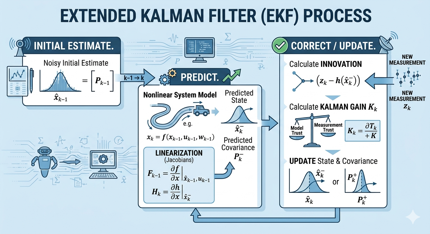
Linearization Using Jacobians
Since the system is nonlinear, we compute Jacobians:
State Transition Jacobian
\[ F_k = \left.\frac{\partial f}{\partial x}\right|_{\hat{x}_{k-1|k-1}, u_k}\]
Measurement Jacobian
\[ H_k = \left.\frac{\partial h}{\partial x}\right|_{\hat{x}_{k|k-1}}\]
EKF Algorithm
The EKF consists of two steps: Prediction and Update.
1. Prediction Step
State Prediction
\[ \hat{x}_{k|k-1} = f(\hat{x}_{k-1|k-1}, u_k)\]
Covariance Prediction
\[ P_{k|k-1} = F_k P_{k-1|k-1} F_k^T + Q_k\]
2. Update Step
Innovation
\[ y_k = z_k - h(\hat{x}_{k|k-1})\]
Innovation Covariance
\[ S_k = H_k P_{k|k-1} H_k^T + R_k\]
Kalman Gain
\[ K_k = P_{k|k-1} H_k^T S_k^{-1}\]
State Update
\[ \hat{x}_{k|k} = \hat{x}_{k|k-1} + K_k y_k\]
Covariance Update
\[ P_{k|k} = (I - K_k H_k) P_{k|k-1}\]
Differences from Standard Kalman Filter
| Feature | Kalman Filter | Extended Kalman Filter |
|---|---|---|
| Model | Linear | Nonlinear |
| Matrices | Constant | Jacobians |
| Accuracy | Optimal | Approximate |
| Complexity | Low | Higher |
Key Insights
Linearization Error
EKF uses first-order approximation:
- Works well for mild nonlinearities
- Can diverge for strong nonlinearities
Importance of Jacobians
Accurate Jacobians are critical for performance.
Consistency Issues
EKF may become overconfident if not tuned properly.
Practical Example: Spacecraft Attitude Estimation
In spacecraft systems:
- State → Quaternion + gyro bias
- Process → Nonlinear attitude dynamics
- Measurement → Star tracker
EKF fuses sensor data to estimate attitude and bias.
EKF Pseudocode
// Prediction
x_pred = f(x, u);
F = Jacobian_f(x, u);
P_pred = F * P * F.transpose() + Q;

// Update
H = Jacobian_h(x_pred);
y = z - h(x_pred);
S = H * P_pred * H.transpose() + R;
K = P_pred * H.transpose() * inverse(S);

x = x_pred + K * y;
P = (I - K * H) * P_pred;